Text to image generation Using Deep Convolution Generative Adversarial Networks (DCGANs)

Objectives:

1. To generate realistic images from text descriptions.

2. To use the skip thought vector encoding for sentences.

3. To construct Deep Convolutional GAN and train on MSCOCO and CUB datasets.

Related Theoritical concepts

A. Skip-Thought Vectors

Skip-thought model [1] is an unsupervised encoder-decoder model for encoding large chunks of text irrespective of the application domain. This approach is novel in the sense of shift from compositional semantics based methods, while maintaining the same quality. The input to this model, while training, is a tuple of sentences . The encoder generates a state vector corresponding to words of the sentence at time step . One of the two decoders predicts the word in the next sentence and the other decoder predicts the word in previous sentence from the current state vector . The objective function is sum of log probabilities of forward and backward sentences given the encoder representation

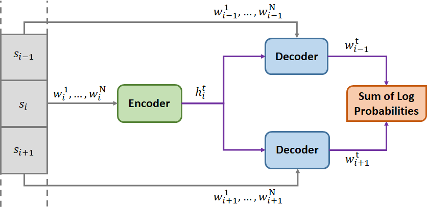
In simpler terms, maximizing the sum of log probabilities would lead to generation of a faithful state vector which encodes information required to make predictions about the nearby sentences.

Another important feature proposed in [2] is vocabulary expansion. The vocabulary for this RNN based model, represented as , is relatively small as compared to other representations like word2vec, represented by . A transformation can constructed such that , such that by minimizing L2 loss to obtain W.

B. Generative Adversarial Networks

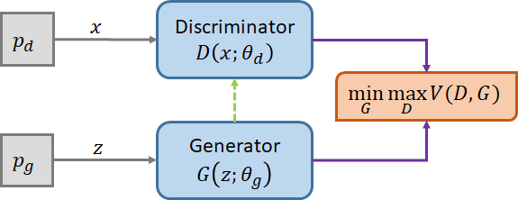
Generative Adversarial Networks (GAN) [2] consists of a generator G responsible for generating examples from noise distribution , parameterized by , which are similar to the data distribution and a discriminator D, responsible for distinguishing the examples arising from the data distribution , parameterized by , against those generated by G.

The requirements for this framework to generate examples indistinguishable from the data distribution are:

1. The discriminator D should maximise the probability of correctly classifying the the source of examples.

2. The generator G should maximise the probability that D incorrectly classifies the the generated examples.

This is a minimax game between G and D as:

The training of GANs is difficult and success of GANs has been demonstrated by using MLP based generators and discriminators. It is observed that discriminator can be safely trained while generator is halted, but training generator while discriminator is halted leads to Mode Collapse [3] where generator generates almost identical images which can deceive the discriminator. Hence, the training of discriminator and generator has to go hand in hand.

C. Generative Adversarial Text to Image Synthesis

Caption to image generation has been addressed in [4]. The underlying idea is to augment the generator and discriminator in a GAN with suitable text encoding of the description. Conceptually, this is similar to conditioning the operation of the generator and discriminators on the text descriptions. The original work describes the implementation using Deep Convolutional Neural Networks hence the name DCGAN. The generator is a deconvolution network which generates an image from the text based on noise distribution. The discriminator is a convolutional network which outputs the probability of the input image belonging to the original data distribution given the text encoding.

It is the loss function of the network that we changed in to get varying results. As already mentioned the discriminator is a Convolutional Neural Network which was trained on two aspects:

1. It should be able to differentiate between a generated image and an original image for the same image description in text

2. The discriminator should be able to differentiate between a real image and fake text

The naive GAN involves the discriminator network understanding to differentiate between a realistic image and fake text and unrealistic image and original text. As pointed out in [4] we note that this might lead to training complications. Therefore we modify the loss function of the discriminator to include one more source of loss where we penalise the discriminator when it is fed with realistic images with fake text. This technique called Matching Aware GAN therefore includes three parts in the loss functions:

1. Realistic images with original text

2. Unrealistic images with original text

3. Realistic images with fake text

Implementation

We now mention the DCGAN architecture that we have used for our training. Further modifications that have been made are mentioned thereafter.

Before diving into architecture, it is worth noting that the inaccuracies in text encoding could affect the results drastically. Hence, text descriptions were encoded using a pre-trained model for skip-thought vectors as spending resources on training a text encoder from scratch is only secondary to the scope of this project. From implementation point of view, this decision is justifiable as the versatility of this model due to vocabulary expansion can address any scalability issues arising at a later stage.

A Generator Architecture

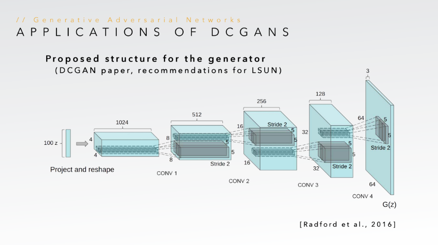
1. After noise is appended to the encoded sentence, we use a deconvolutional neural network (referred to as convolutional nets with fractional strides in [6]). We use 5 layers for the Generator network which are described as follows:
2. Generate 128 dimensional conditioning latent variable using twofully connected layers to map from 4800 dimensional sentence encoded vector to mean and sigma predictions.
3. Sample epsilon from normal distribution and generate the conditioning variable.
4. Append conditioning variable with noise latent variable which is 100 dimensional.
5. Map the appended vector into 4x4x1024 tensor using a fully connected layer and reshape the same.
6. A deconvolutional layer with filter dimension 3x3. Stride length of 2 is used giving an output of 8x8x512. Leaky ReLU activation is used with the slope as 0.3 as suggested in [7]. Padding used is ‘SAME’. The output is batch normalized.
7. A deconvolutional layer with filter dimension 3x3. Stride length of 2 is used giving an output of 16x16x256. Leaky ReLU activation is used with the slope as 0.3. Padding used is ‘SAME’.The output is batch normalized.
8. A deconvolutional layer with filter dimension 3x3. Stride length of 2 is used giving an output of 32x32x128. Leaky ReLU activation is used with the slope as 0.3. Padding used is ‘SAME’.The output is batch normalized.
9. A deconvolutional layer with filter dimension 3x3. Stride length of 2 is used giving an output of 64x64x3. Sigmoid activation is used in this layer. Padding used is ‘SAME’.

B Discriminator Architecture

1. Map the sentence vector into 4x4x128 tensor using a fully connected layer and reshape the same.

2. A convolutional layer with filter dimension 3x3 over the input image. Stride length of 2 is used giving an output of 32x32x64. Leaky ReLU activation is used with the slope as 0.3. Padding used is ‘SAME’. Dropout with keep probability 0.7 was used.

3. A convolutional layer with filter dimension 3x3 over the input image. Stride length of 2 is used giving an output of 16x16x128. Leaky ReLU activation is used with the slope as 0.3. Padding used is ‘SAME’. Dropout with keep probability 0.7 was used.

4. A convolutional layer with filter dimension 3x3 over the input image. Stride length of 2 is used giving an output of 8x8x256. Leaky ReLU activation is used with the slope as 0.3. Padding used is ‘SAME’. Dropout with keep probability 0.7 was used.

5. A convolutional layer with filter dimension 3x3 over the input image. Stride length of 2 is used giving an output of 4x4x512. Leaky ReLU activation is used with the slope as 0.3. Padding used is ‘SAME’. Dropout with keep probability 0.7 was used.

6. Outputs from 1 and 5 are augmented along channels.

7. A convolutional layer with filter dimension 3x3 over the input image. Stride length of 2 is used giving an output of 1x1x1024. Leaky ReLU activation is used with the slope as 0.3. Padding used is ‘SAME’. Dropout with keep probability 0.7 was used.

8. Reshaped to a one dimensional vector and then converted to a single value using a fully connected layer. No activation used in order to use tf.sigmoid_cross_entropy_with_logits() to generate a probability implicitly

C. Loss Functions

The cross-entropy loss function that we use for the discriminator network forces it to produce 1 when a correct image sentence pair is given to it and 0 otherwise. However such hard outputs is generally not desirable for training the discriminator network. This is because for a correct image-sentence pair the discriminator may try to push its output to 1 even when it is actually giving 0.9 as output (say). Therefore we modify the cross-entropy loss function slightly by requiring it to give an output of 0.9 when sentence-image pair is correct and 0.1 otherwise. This technique has been called “Level-Smoothing”.

The losses used for the generator network include the obvious binary cross entropy loss with level smoothened probabilities. In addition to this loss, KL divergence between the conditioning latent variable distributed over mean and variance predicted by initial layers of the generator network and the zero mean unit variance normal distribution is taken. This follows from the reparameterization trick. Also the lagrange multiplier of 2.0 for the KL divergence loss follows from [7].

D. Batch Normalization

As Xavier weight-initialization and ReLu activation functions helps counter the vanishing gradient problem, Batch Normalization is another method for handling the problem of vanishing gradient as well as exploding gradients. Batch Normalization is a method to reduce internal covariate shift in deep neural networks, which leads to the possible usage of higher learning rates [8]. After normalizing the input in the neural network, we don’t have to worry that the scale of input features might be vastly different. Thus, the gradient descent can reduce the oscillations when approaching the minimum point and converge faster. Again Batch Norm also reduces the impacts of earlier layers on the later layers in deep neural network. Beside all the positive effects, still a side-effect of Batch Normalization is regularization. By using mini-batch size, a minor noise will be added to each layer, which imposes the regularization effects. But the regularization effects decrease with larger batch size since the noise diminishes.

E. Reparameterization Trick.

The reparameterization trick is used to transform the encoded sentence vector to a conditional variable needed for the Generator. As we have seen in the Variational Autoencoder setup, the reparameterization trick helps us in enabling the gradients flow through a stochastic node. This also helps mitigate the learning problems from an encoder output space which is ginormous and the vectors of concern might be in sparse and discontinuous subspaces. Thus the space is converted to simple space (normally distributed) to make the task of learning easier.

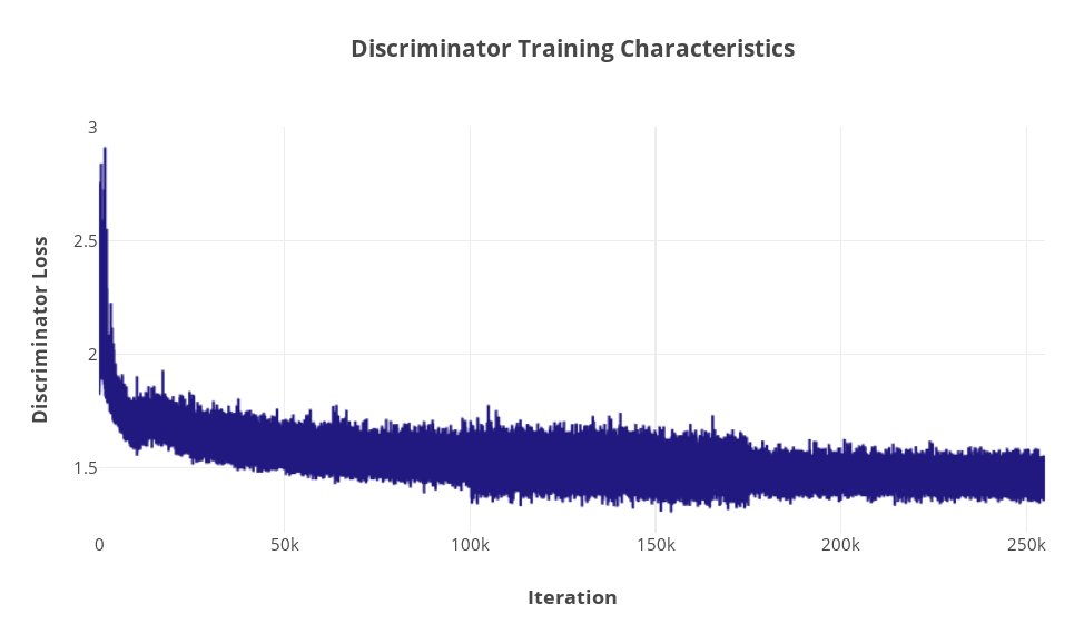
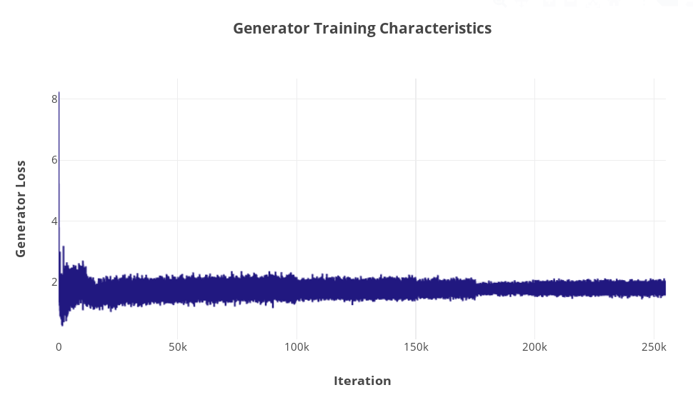
F. Training Curves

Approaches:

A. Without Batch Normalization

Depth of the Generative Network was varied (its depth was always <= depth of the Discriminator network). Since it is generally better if the Discriminator network is better trained than the Generator, we changed the architecture keeping in mind that the final loss of the discriminator should be less than that of the generator. This was however very difficult to achieve while training with MS-COCO dataset.

The model sizes we made were restricted by the GPU’s we used.

B. With Batch Normalization

Once Batch Normalization was added, the training was much faster. We could train the model on the MS-COCO dataset for a batch size of upto 8 on one of the machines. We noticed the introduction of noise as batch normalization was done for smaller batch sizes. Having batch sizes of greater than 8 was not feasible for the machine that we were using for this training.

A. Batch Normalization and Conditional Augmentation

This approach proved to be the best in generating low resolution images. The idea was based on the Stage I implementation of StackGAN and the model was created using the description in the same implementation. Also, high resolution images could be generated by using a SRGAN (Super Resolution GAN ) as Stage II of the same but due to lack of resources and time we could not train the model.

The key aspect of this approach was to use reparameterization trick and generate a continuous and more meaningful distribution out of the encoded sentence vectors before augmenting it with noise to feed in the generator’s decoder part. This has shown that the generated images follow the description better.

Experiments

A. Code Description

This project was developed in Python 3.5 using tensorflow-gpu v1.50, numpy, and pickle. Total length of the codes are roughly 225 lines for each approach followed. This implementation started off with a Conditional GAN made by one of the team members for his graduate seminar.

The source for the implementations discussed in this report is available at:

https://github.com/ayansengupta17/GAN

https://github.com/yagneshbadiyani/C2I

B. Experimental Platform

The experiments were carried out on two Intel Xeon machines with GPUs. One of the machines had a Nvidia GeForce GTX 750 Ti and 8 GB RAM while the other had Nvidia GeForce GTX 1080 Ti (12GB)

The runtime was observed to be approximately 24 hours for majority of the trials carried.

C. Experimental Results

1. DCGAN with Batch Normalization and Conditional Augmentation on CUB

Sentence	Generated Image	Match from Dataset
This little bird has a yellow green colored body, a small black tipped bill and a black crown.
This bird has a white and brown breast with a sharp pointed bill.
This bird is bright red colored with black wings and a small beak.
This bird has a blue crown, blue primaries, and blue secondaries.
This is a small black and white bird with prominent crown feathers.

It can be seen from above pictures how the reparameterization trick plays its role in generating images closer to the description provided.

2. DCGAN without Batch Normalization trained on MS-COCO

Sentence	Generated Image	Match from Dataset
This person is surfing in the ocean during high tide in the afternoon.
A person in white uniform is swinging a baseball bat.

3. DCGAN with Batch Normalization trained on MS-COCO

Sentence	Generated Image	Match from Dataset
Two children with black jackets and white jeans are skating on ice.
A person is surfing in the ocean on a clear day.

We see that the results are much better for the CUBS dataset as compared to the MS-COCO dataset. This might be because of the variability in the MS-COCO dataset.

References

1. Kiros, Ryan, et al. “Skip-thought vectors.” Advances in neural information processing systems. 2015 Link

2. Goodfellow, Ian, et al. “Generative adversarial nets.” Advances in neural information processing systems. 2014. Link

3. Salimans, Tim, et al. “Improved techniques for training gans.” Advances in Neural Information Processing Systems. 2016. Link

4. Reed, Scott, et al. “Generative adversarial text to image synthesis.” arXiv preprint arXiv:1605.05396 (2016). Link

5. Zhang, Han, et al. “Stackgan: Text to photo-realistic image synthesis with stacked generative adversarial networks.” IEEE Int. Conf. Comput. Vision (ICCV). 2017. Link

6. Alec Radford, Luke Metz, and Soumith Chintala. “Unsupervised representation learning with deep convolutional generative adversarial networks.” arXiv preprint arXiv:1511.06434, 2015. Link

7. Diederik P Kingma and Max Welling.” Auto-Encoding Variational Bayes.” International Conference on Learning Representations (ICLR), 2014. Link

8. Sergey Ioffe, Christian Szegedy, “Batch Normalization: Accelerating Deep Network Training by Reducing Internal Covariate Shift.” arXiv preprint arXiv:1502.03167v3 (2015) Link

Other Important Resources

1. Ian Goodfellow: Generative Adversarial Networks (NIPS 2016 tutorial)

2. NIPS 2016 Workshop on Adversarial Training - Ian Goodfellow - Introduction to GANs
3. DCGAN
4. Skip-thought vectors